Powder particle size distribution-PSD introduce

1. Definition

Particles in a sample of powder don't have all the same size. In order to characterize the solids for some applications where the size is an important parameter, it is necessary to measure the size of the population of the particles and describe which proportion of the sample corresponds to a given size (or range of size). The result of the analysis is usually presented in 2 formats : a cumulative distributino and a frequency (or differential) distribution.

2. Calculation

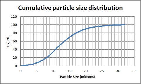
The cumulative particle size distribution is showing for each size of particles which % of the sample has a size lower or equal.

Picture 1 : Cumulative distribution

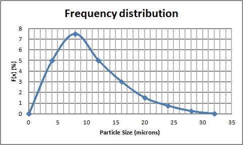
The frequency particle size distribution (or differential) is showing which % of a sample corresponds to a given diameter (it can also be a range of diameters).

Pic 2 : Frequency distribution


It is possible to get the cumulative distribution by integration of the frequency distribution. Thus, it is possible to get the frequency distribution by derivation of the cumulative distribution.

The distribution can be of different type according to the way to count the population. The size distribution can be as a function of :
- Number of particles
- Length
- Surface
- Volume (or weight)

It is actually possible (although not very accurate) to go from one distribution to another thanks to a shape factor.

It is often required to find characteristic measures of the distribution. Most of the time it will consist in finding a characteristic diameter. One way is to look for a mean diameter, but it must be noted that there are different ways to calculate mean diameters that will be more or less relevant depending on the application. 2 mean diameters that are often used to characterize a distribution are given below :

Equation 1 : Mean diameters for PSD characterization

Another practical method is to use the d50 and d90, they correspond to the diameters for which 50% and 90% of the sample will have a diameter lower that the determined d50 and d90.

3. Measurement of particle size distribution PSD

Different methods, more or less complicated and accurate can be used to determine a particle size distribution. 2 methods often used are described below.

Basic method : sieving

A popular method, since it does not request large investments, is to use a sieving tower. The tower is made of different wire mesh sieves, going finer and finer. The sample is placed at the top of the tower and the system is put on vibration. After a defined vibration time, the quantity collected at each sieve is weighed. An histogram, corresponding to the frequency particle size distribution of the sample can be drawn.

The method is cheap, fast but rather coarse in the results obtained and can be used mainly for powder that can be easily manipulated.

Figure 1 : Particle Size Distribution by sieving

Advanced method : laser diffraction

Laser diffractometry (also called Fraunhoffer diffraction) is an automated and accurate method to determine the PSD of a sample. Such method required to put in suspension the solids, which may not be possible for all kind of solids (dissolution - different kind of liquid can however be used). A laser beam is passed through the sample, the intensity and of the light diffracted and the angle of diffraction allow to measure the size of the particles and count their number.

Note : all methods have pros and cons and the interpretation of the result must be done by people understanding the limits and hypothesis of each method.

4. Application of PSD

Knowing the PSD of a sample can be important to drive a process or even release a production from a quality point of view. Typical processing requiring PSD at one point or another :
- Milling process
- Granulation process
- Spray Drying process
- Crystalization process
Typically all processes where a calibrated powder is required.

The frequency distribution gives interesting information about the population of particles. Quite commonly, there is a single peak in the distribution. The particle is then said monomodal. But is can also happen that there are several peaks, in this case the distribution is said multimodal. In the case of a milling process for example, the appearance of a 2nd peak can show that the mill is not performing as foreseen.

It can also be interesting to model the distribution by a law :
- Normal 
- Log-Normal 
- Rosin Rammler

Each representation can be useful for subsequent calculations, or to determine when the sample is abnormal (it does not fit the law that can model this kind of samples).

LAST：Vacuum Pneumatic transport feeding machine introduction

NEXT：Powder and Gas separation Introduce(cyclone - filtration)